Efficiency Measurement and Data Envelopment Analysis (DEA)

Kabui, Charles

Open in Kaggle Download as Notebook Download as PDF

Efficiency Measurement and Data Envelopment Analysis (DEA)

Efficiency measurement is about quantifying how well an entity, such as a company, department, or individual,uses its resources (inputs) to achieve its goals (outputs). The aim is to maximize outputs while minimizing inputs, ensuring optimal use of available resources.

Data Envelopment Analysis (DEA) is a non-parametric mathematical method used to measure the relative efficiency of a set of similar decision-making units (DMUs). DEA evaluates each DMU by comparing its inputs and outputs, using a ratio of the weighted sum of outputs to the weighted sum of inputs. This makes it ideal for assessing efficiency when multiple inputs and outputs are involved.

DEA has numerous real-world applications, including:

Healthcare: Evaluating hospitals based on inputs like the number of doctors, nurses, and beds, versus outputs such as the number of patients treated or survival rates, with the goal of identifying underperforming facilities
Banking: Assessing bank branches by comparing inputs like staff size and operating costs against outputs such as new accounts opened or loans processed, aiming to optimize branch operations
Education: Measuring schools’ efficiency by comparing inputs like teachers, classroom space, and funding against outputs like test scores and graduation rates, to improve educational outcomes and resource allocation.
Energy Sector: Analyzing the efficiency of power plants by comparing fuel and labor inputs to energy output and environmental impact, with the goal of minimizing waste and enhancing sustainability
Public Sector: Evaluating local governments or public services (e.g., waste management, policing) to ensure effective and efficient use of public funds

Types of DEA Models

There are several DEA models, each suited to different scenarios:

The CCR model (Constant Returns to Scale) assumes that a proportional increase in inputs will result in a proportional increase in outputs. It is often used as a baseline for efficiency comparisons
The BCC model (Variable Returns to Scale) allows for cases where outputs do not necessarily change proportionally with inputs, accommodating increasing, constant, or decreasing returns to scale

DEA Orientations

DEA models can also be classified by their orientation:

Input-oriented models focus on minimizing the inputs required to produce a given level of outputs
Output-oriented models aim to maximize the outputs achieved with a given set of inputs
Non-oriented models are used when both input reductions and output increases are desired simultaneously

Other advanced DEA variants include Two-Stage DEA, Slack-Based Measure (SBM), Network DEA, Super-Efficiency DEA, Fuzzy DEA, and Stochastic DEA, each addressing specific analytical needs.

Basic DEA Model: CCR Input-Oriented

The basic DEA model (CCR Input-Oriented) is designed to minimize input usage while maintaining at least the current level of outputs. It operates under the assumption of constant returns to scale. The objective is to determine how much each decision making unit (DMU) can proportionally reduce its inputs without reducing outputs, while ensuring that no other DMU performs better. The model outputs an efficiency score ranging from 0 to 1:

A score of 1.0 signifies full efficiency.
A score below 1 indicates potential for improvement.

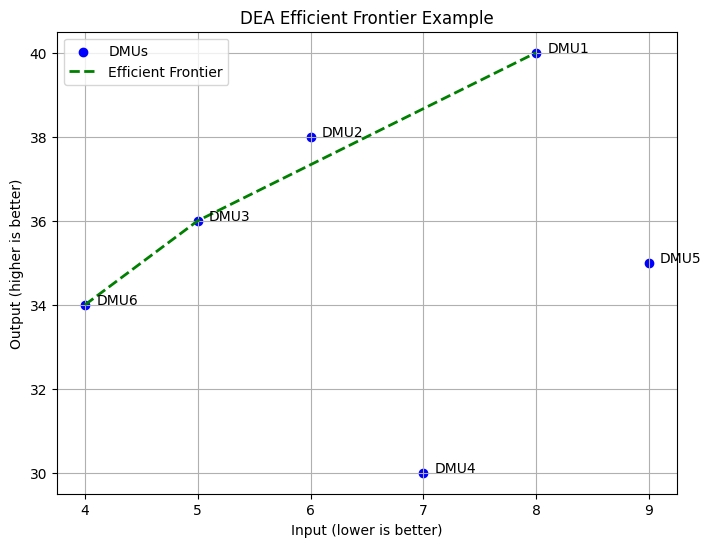
Visualizing DEA: The Efficient Frontier

A graphical illustration can help visualize DEA by plotting DMUs with input on one axis and output on the other. The efficient frontier is formed by connecting the most efficient DMUs, representing those producing the most output for the least input. DMUs below the efficient frontier are considered inefficient as they use more input than necessary for their output level. This visualization helps identify best and lagging units.

import numpy as np
import matplotlib.pyplot as plt

# Sample DMU data: Inputs (lower is better), Outputs (higher is better)
inputs = np.array([8, 6, 5, 7, 9, 4])
outputs = np.array([40, 38, 36, 30, 35, 34])
names = ['DMU1', 'DMU2', 'DMU3', 'DMU4', 'DMU5', 'DMU6']

# Plot DMUs
plt.figure(figsize=(8, 6))
plt.scatter(inputs, outputs, color='blue', label='DMUs')

# Annotate DMUs
for i, name in enumerate(names):
    plt.annotate(name, (inputs[i]+0.1, outputs[i]))

# Efficient frontier (manually connecting the efficient DMUs)
# Let's assume DMU6, DMU3, and DMU1 are efficient
frontier_inputs = [4, 5, 8]
frontier_outputs = [34, 36, 40]
plt.plot(
  frontier_inputs, 
  frontier_outputs, 
  color='green', 
  linestyle='--', 
  linewidth=2, 
  label='Efficient Frontier')

plt.title('DEA Efficient Frontier Example')
plt.xlabel('Input (lower is better)')
plt.ylabel('Output (higher is better)')
plt.legend()
plt.grid(True)
plt.show()

Practical DEA Tools: Benchmarking with R vs. Python

While pyDEA is an open-source Python package designed for conducting DEA, in practice, it has significant limitations. Although it supports standard models like CCR and BCC and accepts CSV input, pyDEA is cumbersome to set up, lacks flexibility for interactive analysis, and is difficult to integrate into practical workflows.

R offers a more mature and practical ecosystem for DEA through packages like Benchmarking. The Benchmarking package is widely used in academia and industry for DEA and provides:

Support for both CCR and BCC models
Flexible handling of input- and output-oriented approaches
Functions to compute efficiency scores, reference sets, and slacks
Simple integration with data frames and visualization tools
Ease of scripting and automation for batch efficiency evaluations

Because of its robustness, ease of use, and flexibility, Benchmarking with R is generally considered the best practical tool for efficiency measurement using DEA. It is especially well-suited for professionals and researchers who need accurate, transparent, and reproducible results.

Examples

Hospital Department Efficiency

You are analyzing the performance of 4 hospital departments. Each department has a different combination of medical staff and beds. You want to know: Which department is most efficient in treating patients with limited resources?

Inputs:

Doctors: [40, 35, 45, 38]
Nurses: [80, 70, 85, 75]
Beds: [150, 140, 160, 145]

Outputs:

Patients treated: [2,000, 1,900, 2,100, 1,950]
Survival rate: [0.97, 0.96, 0.98, 0.95]

Answer

%%R

# install.packages("Benchmarking")
library(Benchmarking)
library(knitr)

# Function to create efficiency table
generate_efficiency_table <- function(names, scores, unit_label = "Unit") {
  # Calculate interpretation text
  interpretation <- ifelse(
    scores == 1,
    "Fully efficient (benchmark unit)",
    paste0("Can reduce inputs by ~", round((1 - scores) * 100, 1), "%")
  )
  
  # Create dataframe
  df <- data.frame(
    unit_label = names,
    Efficiency_Score = round(scores, 3),
    Interpretation = interpretation,
    stringsAsFactors = FALSE
  )

  colnames(df)[1] <- unit_label  # Dynamic column name
  
  # Print the dataframe
  kable(df)
}

%%R

# Inputs: Doctors, Nurses, Beds
inputs <- matrix(
  c(40, 80, 150,
    35, 70, 140,
    45, 85, 160,
    38, 75, 145),
  nrow = 4,
  byrow = TRUE
)

# Outputs: Patients treated, Survival rate
outputs <- matrix(
  c(2000, 0.97,
    1900, 0.96,
    2100, 0.98,
    1950, 0.95),
  nrow = 4,
  byrow = TRUE
)

# Run DEA (input-oriented, constant returns to scale)
dea_result <- dea(X = inputs, Y = outputs, RTS = "crs", ORIENTATION = "in")

# Print efficiency scores
print(dea_result$eff)

names <- c("Dept 1", "Dept 2", "Dept 3", "Dept 4")

# Generate table
generate_efficiency_table(names, dea_result$eff, "Department")

[1] 0.9824561 1.0000000 0.9671053 0.9909256


|Department | Efficiency_Score|Interpretation                   |
|:----------|----------------:|:--------------------------------|
|Dept 1     |            0.982|Can reduce inputs by ~1.8%       |
|Dept 2     |            1.000|Fully efficient (benchmark unit) |
|Dept 3     |            0.967|Can reduce inputs by ~3.3%       |
|Dept 4     |            0.991|Can reduce inputs by ~0.9%       |

Department 2 is the benchmark performer, operating fully efficiently by maximizing patient outcomes with its available staff and beds. In contrast, Department 3 is the least efficient, with potential to reduce its resource use by about 3.3% while maintaining the same output. Department 3 should be reviewed more closely - check if it’s overstaffed, underperforming, or facing operational issues. Departments 1 and 4 are close to efficiency but still have minor room for optimization.

Retail Store Efficiency

A retail company wants to assess whether its 4 branches are efficiently turning staff and marketing investment into profit. Which store branch is the best performer given similar resource levels?

Inputs:

Marketing Spend (USD): [$12,000, $10,000, $11,500, $9,800]
Employees: [20, 18, 22, 19]

Outputs:

Monthly Revenue (USD): [$110,000, $100,000, $120,000, $95,000]
Number of Customers: [2,300, 2,000, 2,600, 1,900]

Answer

%%R

# Inputs: Marketing Spend (USD), Employees
inputs <- matrix(
  c(12000, 20,
    10000, 18,
    11500, 22,
    9800, 19),
  nrow = 4,
  byrow = TRUE
)

# Outputs: Monthly Revenue (USD), Number of Customers
outputs <- matrix(
  c(110000, 2300,
    100000, 2000,
    120000, 2600,
    95000, 1900),
  nrow = 4,
  byrow = TRUE
)

# Run DEA (input-oriented, constant returns to scale)
dea_result <- dea(X = inputs, Y = outputs, RTS = "crs", ORIENTATION = "in")

# Print efficiency scores
print(dea_result$eff)

names <- c("Store 1", "Store 2", "Store 3", "Store 4")

# Generate table
generate_efficiency_table(names, dea_result$eff, "Branch/Store")

[1] 1.0000000 1.0000000 1.0000000 0.9289966


|Branch/Store | Efficiency_Score|Interpretation                   |
|:------------|----------------:|:--------------------------------|
|Store 1      |            1.000|Fully efficient (benchmark unit) |
|Store 2      |            1.000|Fully efficient (benchmark unit) |
|Store 3      |            1.000|Fully efficient (benchmark unit) |
|Store 4      |            0.929|Can reduce inputs by ~7.1%       |

Stores 1, 2, and 3 are fully efficient, effectively turning their marketing spend and staff into revenue and customer traffic. In contrast, Store 4 is underperforming, with efficiency at 92.9%, suggesting it could boost its revenue/customers or cut resource use by 7% to match the top performers. Store 4 requires operational review to identify and address gaps in marketing effectiveness or staff productivity.

School Performance Evaluation

A school district monitors 4 schools to find out which one is using its resources most efficiently to produce better academic results.

Inputs:

Teachers: [30, 25, 20, 28]
Annual Budget (USD): [$800,000, $750,000, $700,000, $770,000]

Outputs:

Graduation Rate (%): [85, 90, 82, 88]
Average Test Score (out of 100): [78, 80, 76, 79]

Answer

%%R

# Inputs: Teachers, Annual Budget (USD)
inputs <- matrix(
  c(30, 800000,
    25, 750000,
    20, 700000,
    28, 770000),
  nrow = 4,
  byrow = TRUE
)

# Outputs: Graduation Rate (%), Average Test Score
outputs <- matrix(
  c(85, 78,
    90, 80,
    82, 76,
    88, 79),
  nrow = 4,
  byrow = TRUE
)

# Run DEA (input-oriented, constant returns to scale)
dea_result <- dea(X = inputs, Y = outputs, RTS = "crs", ORIENTATION = "in")

# Print efficiency scores
print(dea_result$eff)

names <- c("School 1", "School 2", "School 3", "School 4")

# Generate table
generate_efficiency_table(names, dea_result$eff, "School")

[1] 0.9017857 1.0000000 1.0000000 0.9577922


|School   | Efficiency_Score|Interpretation                   |
|:--------|----------------:|:--------------------------------|
|School 1 |            0.902|Can reduce inputs by ~9.8%       |
|School 2 |            1.000|Fully efficient (benchmark unit) |
|School 3 |            1.000|Fully efficient (benchmark unit) |
|School 4 |            0.958|Can reduce inputs by ~4.2%       |

Schools 2 and 3 are fully efficient, effectively using their teachers and budgets to achieve strong graduation rates and test scores. School 4 is close to efficient but has room to improve by about 4.2%. School 1 is the least efficient, with potential to optimize resources by nearly 10%. School 1 should be prioritized for review and targeted improvements because it either uses more resources than needed or isn’t getting the best academic outcomes relative to its peers.

Disclaimer: For information only. Accuracy or completeness not guaranteed. Illegal use prohibited. Not professional advice or solicitation. Read more: /terms-of-service

Reuse

GNU GENERAL PUBLIC LICENSE v3.0(View License)

Citation

BibTeX citation:

@misc{kabui2025,
  author = {{Kabui, Charles}},
  title = {Efficiency {Measurement} and {Data} {Envelopment} {Analysis}
    {(DEA)}},
  date = {2025-05-08},
  url = {https://toknow.ai/posts/computational-techniques-in-data-science/data-envelopment-analysis/index.html},
  langid = {en-GB}
}

For attribution, please cite this work as:

Kabui, Charles. 2025. “Efficiency Measurement and Data Envelopment Analysis (DEA).” https://toknow.ai/posts/computational-techniques-in-data-science/data-envelopment-analysis/index.html.