Stochastic: Steady-State Probability, Markov Chains and Network Visualization

---

Open in Kaggle Download as Notebook Download as PDF

---

In the world of data science, systems often evolve over time in ways that depend only on their current state - not their entire history. This concept is at the heart of Markov chains, a powerful mathematical tool for modeling sequences of events where the next state depends only on the current one. Whether you’re analyzing user behavior on a website, modeling weather patterns, simulating queues, or building recommender systems, Markov chains offer an elegant and effective way to understand and predict dynamic systems.

At their core, Markov chains rely on transition matrices that define the probability of moving from one state to another. By analyzing these matrices, data scientists can compute steady-state probabilities - a long-term distribution of where the system is likely to be. Simulating these chains also allows us to observe patterns over time and visualize how the system behaves dynamically.

Steady-State Probability Calculation

You are given the following 3×3 transition matrix representing the state changes of a system over time:

P = [
  0.7  0.2  0.1
  0.3  0.4  0.3
  0.3  0.2  0.5
]

Tasks:

1. Represent the matrix in Python using NumPy.
   
2. Verify if this matrix is a valid stochastic matrix.
   
3. Compute the steady-state probabilities analytically using Python.

Answer

Represent the matrix in Python using NumPy

import numpy as np

P = np.array([
    [0.7, 0.2, 0.1],
    [0.3, 0.4, 0.3],
    [0.3, 0.2, 0.5]
])
P

array([[0.7, 0.2, 0.1],
       [0.3, 0.4, 0.3],
       [0.3, 0.2, 0.5]])

Verify if this matrix is a valid stochastic matrix

A stochastic matrix has non-negative entries and each row sums to 1.

# Check non-negativity
is_non_negative = np.all(P >= 0)

# Check if each row sums to 1
row_sums = np.sum(P, axis=1)
rows_sum_to_one = np.allclose(row_sums, 1)

is_valid_stochastic = is_non_negative and rows_sum_to_one
print("Valid stochastic matrix:", is_valid_stochastic)

Valid stochastic matrix: True

Compute the steady-state probabilities analytically using Python

Solve for π such that πP = π and sum(π) = 1

# Solve for steady-state vector π
A = P.T - np.eye(3)
A = np.vstack((A, np.ones(3)))
b = np.array([0, 0, 0, 1])

steady_state = np.linalg.lstsq(A, b, rcond=None)[0]
print("Steady-state probabilities:", steady_state)

Steady-state probabilities: [0.5  0.25 0.25]

Verify πP = π

steady_state

array([0.5 , 0.25, 0.25])

np.array_equal(
    np.round(np.dot(steady_state, P), 2),
    np.round(steady_state, 2))

True

Markov Chain Simulation and Visualization

Using the same transition matrix P in question One, simulate a Markov chain for 50 time steps, starting from state 0.

Tasks:

1. Simulate the Markov chain and record the state at each time step.
   
2. Count how many times each state was visited.
   
3. Plot the sequence of visited states over time using matplotlib.
   
4. Visualize the frequency distribution of states visited using a bar plot.

Answer

Simulate the Markov chain for 50 time steps starting from state 0

def simulate_markov_chain(P, start_state, steps):
    current_state = start_state
    states = [current_state]

    for _ in range(steps):
        current_state = np.random.choice(P.shape[0], p=P[current_state])
        states.append(int(current_state))

    return states

simulated_states = simulate_markov_chain(P, start_state=0, steps=50)

Count how many times each state was visited

from collections import Counter
import pandas as pd

state_counts = dict(Counter(simulated_states))
pd.DataFrame({ 
    "state": state_counts.keys(),
    "visit count": state_counts.values() 
}).set_index("state")

	visit count
state
0	26
1	17
2	8

Plot the sequence of visited states over time using matplotlib

import matplotlib.pyplot as plt

plt.figure(figsize=(10, 4))
plt.plot(simulated_states, marker='o')
plt.title("Visited States Over Time")
plt.xlabel("Time Step")
plt.ylabel("State")
plt.grid(True)
plt.show()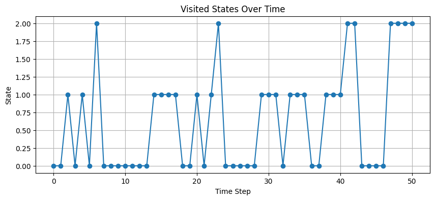

Visualize the frequency distribution of states visited using a bar plot

plt.figure(figsize=(6, 4))
plt.bar(state_counts.keys(), state_counts.values(), color='skyblue')
plt.title("State Visit Frequency")
plt.xlabel("State")
plt.ylabel("Frequency")
plt.xticks([0, 1, 2])
plt.grid(True, axis='y')
plt.show()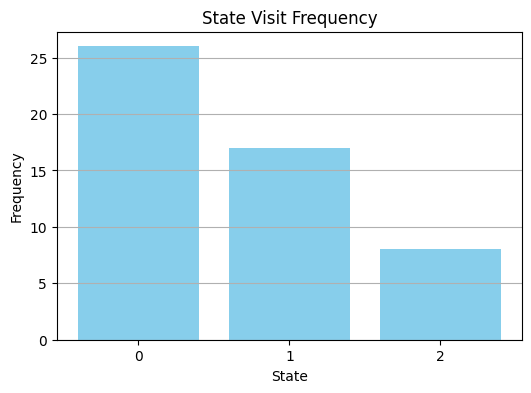

Network Visualization of State Transitions

Using the transition matrix P in question One again, create a directed graph of the Markov chain.

Tasks:

1. Use networkx to create a directed graph where:
   • Nodes represent the states (0, 1, 2).
     
   • Edges represent transitions with weights corresponding to transition probabilities.
     
2. Draw the graph using matplotlib.
   
3. Use edge thickness or labels to indicate the strength of the transition probabilities.

Answer

Create a directed graph using networkx

import networkx as nx

G = nx.DiGraph()

# Add nodes and edges with weights
for i in range(P.shape[0]):
    for j in range(P.shape[0]):
        if P[i, j] > 0:
            G.add_edge(i, j, weight=P[i, j])

Draw the graph using matplotlib with edge labels and thickness

pos = nx.circular_layout(G)
edge_weights = [
    G[u][v]['weight'] * 5 
    for u, v 
    in G.edges()
]

plt.figure(figsize=(6, 6))
nx.draw(
    G, 
    pos, 
    with_labels=True, 
    node_color='lightgreen', 
    node_size=1500, 
    edge_color='gray', 
    width=edge_weights, 
    arrowsize=20)

# Add edge labels
edge_labels = {
    (u, v): f"{d['weight']:.2f}" 
    for u, v, d 
    in G.edges(data=True)
}
nx.draw_networkx_edge_labels(
    G, 
    pos, 
    edge_labels=edge_labels)

plt.title("Markov Chain Transition Graph")
plt.show()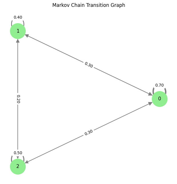

---

Disclaimer: For information only. Accuracy or completeness not guaranteed. Illegal use prohibited. Not professional advice or solicitation. Read more: /terms-of-service